Considering Policy Reversion: The Parity Paradox

 

Historically, challenging times create strong temptation to recycle old policy ideas; a reversion to policies discarded in the past when cyclical problems reappear.  As is well known, recent years have returned relatively lower commodity prices with expectations of more challenging years ahead.  A review of potential reversionary routes would have to begin where farm policy began: parity policy, which was in place from the New Deal 1930s through the 1960s.  That policy proved to be an overwhelming failure throughout its nearly 40-year existence and this article reviews it.

 

 

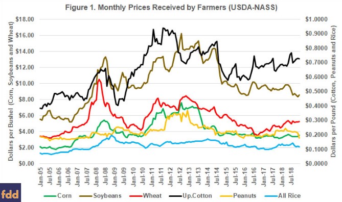
The most recent era for commodity prices would logically trace to 2005 when Congress first enacted the Renewable Fuels Standard (RFS), mandating that increasing volumes of ethanol be blended into the transportation fuel supply (Coppess 2016).  Figure 1 illustrates the monthly prices received by farmers as reported by USDA’s National Agriculture Statistics Service (NASS) Quick Stats web database (https://quickstats.nass.usda.gov/).  Figure 1 covers the RFS period from 2005 to 2018; prices for all rice have been converted from dollars per hundredweight to dollars per pound.

 

 

NASS continues to calculate parity prices, using the monthly prices received and converted to the indexes for the parity base period (1910-1914 = 100) to compute the parity prices and ratios, also available on the Quick Stats web database.  The operative definition is contained in the Code of Federal Regulations and states that parity is the “index of prices paid by farmers, interest, taxes, and farm wage rates” and the “measure of the general level of prices received by farmers” over the preceding 10 calendar years with adjustments (7 C.F.R. §5.1).  Figure 2 illustrates the monthly price received by farmers for each of the commodities as a percent of the parity price calculated by USDA.

 

 

It is notable that, as currently calculated, not a single commodity is above 40% of the parity price.  No commodity reached 100% of parity during the entire RFS-influenced price era.  The highest was wheat at 84% of parity in March 2008.

 

 

One definition of paradox is “an argument that apparently derives self-contradictory conclusions by valid deduction from acceptable premises” (Merriam-Webster.com).  As originally conceived in 1933 and revised in 1938, the New Deal parity policy was designed to restore the purchasing power of agricultural commodities; to improve prices for farmers in the depths of depression by managing supply and providing price supporting loans (Coppess, 2018).  It was accepted that farmers, like the rest of the economy at the time, were in depression and that prices for crops had been too low as compared to what it cost to produce the crop.  In fact, the farm economic problems had predated the Great Depression by over a decade; commodity prices went into a depressed state in the aftermath of World War I.

 

Among the more puzzling aspects of parity policy—aside from its survival through decades of failure—was the way the policy sought to address these economic problems.  It was rooted in a conclusion that farming should operate more like industry, controlling its supplies when prices were low in order to improve them or until stronger demand improved prices.  One problem with this as applied to farming, however, was that there were millions of farmers making independent decisions and in competition with each other, as well as farmers around the world (not to mention the overwhelming impact of weather).  In place of industry’s ability to calibrate production to demand, parity policy placed the federal government in the role of trying to balance supplies and demand.  Controlling supplies of the major commodities at levels that would just meet domestic demand and some export needs, but to avoid shortages, proved to be an impossible task.  Problems with the policy began with the fact that the mechanism of control was through a reduction of acres that farmers were permitted to plant (e.g., acreage allotments).  The policy touched off a set of intractable problems in addition to the economic problems confronting farmers.  Designed to manage or control supplies, perspective on parity policy begins there.

 

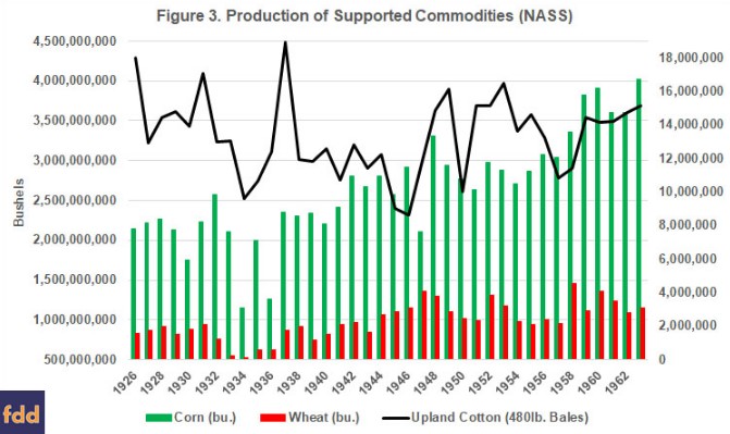
According to NASS data, production was initially reduced upon implementation of the parity system, but it fluctuated greatly and increased over time, especially after World War II.  Figure 3 charts the production data from NASS beginning with the pre-parity years before the Agricultural Adjustment Act of 1933 (1926-1932) and continuing through 1963, as the system broke down completely.

 

 

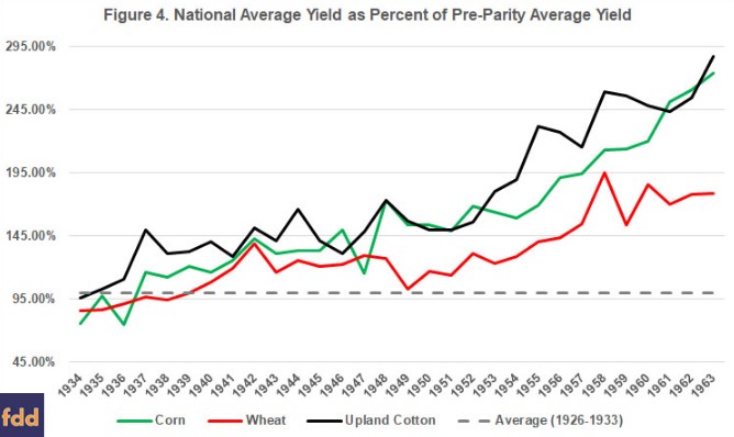
One of the biggest problems for the parity system’s attempts to control or manage supplies—aside from the completely unpredictable nature of weather during the growing season and after estimates were made for allotments—was that per-acre crop yields for the supported commodities increased significantly during the era of parity policy.  Figure 4 illustrates this increase in yields, comparing the national average crop yield, as reported by NASS data, with the national average yields during the pre-parity years (1926 through 1933).  As is evident, yields began to increase significantly after World War II, with adoption of mechanization, hybrid seeds and chemical inputs, especially synthetic fertilizers.  For example, wheat yields were around 11 or 12 bushels per acre when the parity system was created.  By the time wheat farmers rejected supply controls in the 1963 wheat referendum, wheat yields were 25 bushels per acre (179% of the 1926-1933 average).  Similarly, cotton yields were 213 pounds per acre in 1933 but had increased to 517 pounds per acre by 1963 (288% of the 1926-1933 average).  In both cases, efforts to reduce supplies by reducing acres would have required about half the acres planted to each crop; a reduction in acreage so steep as to be politically untenable.

 

 

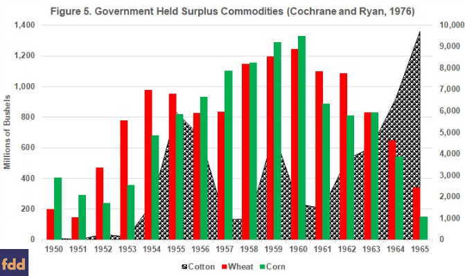
The parity policy experience taught that it is nearly impossible for policy to control or manage supplies of these commodities, especially over any significant number of years.  Weather and farm practices (mechanization, hybrids, chemicals and fertilizers) have far more impact on supplies.  Limiting acres, moreover, tends to incentivize farmers to increase yields on the acres that remain in production, especially when limits on acres are coupled with price-based assistance.  The end result was a failure to control supplies and large surpluses being held by the federal government; forfeited by farmers under the parity loan (price support) policy, these federal stores of commodities were a very public reminder that the policies were not working.  Figure 5 illustrates the total surplus commodities held by USDA during the key post-war years (Cochrane and Ryan, 1976).

 

 

In addition to not being able to effectively control or manage supplies, the parity policy’s use of acreage allotments and reductions fueled a series of additional problems.  Total acres of the major commodities did not change drastically from 1926 through at least 1956 when Congress created the Soil Bank and the Conservation Reserve Program (farmdoc daily, May 4, 2017).  According to NASS data, total acres planted to these crops from 1926 to 1933 averaged over 280 million.  From the onset of parity through the U.S. entry in World War II in 1941, total average acres were nearly 277 million acres.  And during the ten years after World War II, and before the Soil Bank (1947-1956), total acres planted to these crops averaged 271 million acres.  This indicates that few acres came out of production, even as yields were increasing; instead, acres shifted among the major commodities.  Figure 6 illustrates the acres planted each year from 1926 through 1963 of the major commodities, including soybeans and the other feed grains (barley, oats, rye and sorghum); soybeans were not part of the parity system.

 

 

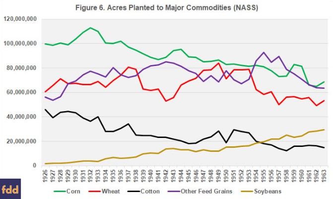
Aside from the steady increase in soybean acres, Figure 6 also illustrates the political problems the parity acreage allotment system caused.  As acres of supported commodities were significantly reduced, many acres shifted to soybeans but also to the other feed grains (barley, oats, rye and sorghum).  These other feed grains would compete with corn for the lucrative domestic feed market; a situation most notable beginning in 1954 when acres in the other feed grains (purple line) surpassed acres in corn (green line).  This acreage shift continued until corn farmers voted to leave the system in 1959, and it magnified political tension between the regional competitors in the Midwest and the South.  That political tension, in turn, complicated Congressional efforts to write, revise and pass farm policy during the 1950s and 1960s (Coppess, 2018).

 

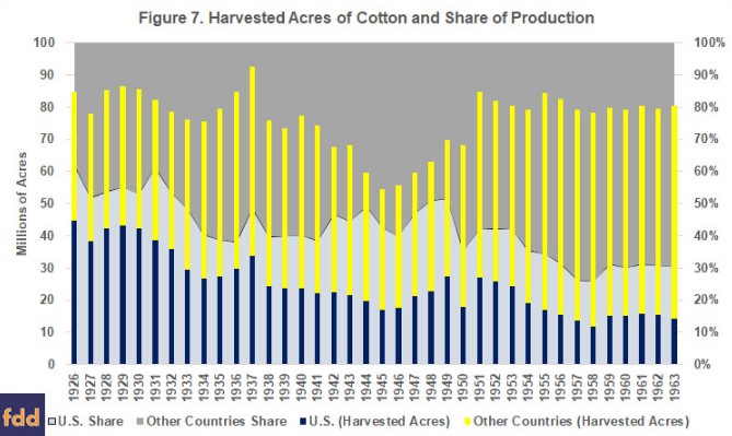
In addition to fueling domestic political problems, the parity system’s policy of reducing acres planted to supported crops in the United States had impacts beyond our borders.  These commodities are staples produced around the world and traded in world markets.  Acres reduced in America can be offset by increased acres and production by farmers in other countries, a problem that the parity system laid bare.  Arguable, cotton provided the strongest example given its large dependence on export markets.  Figure 7 illustrates the cotton issue as reported by the Senate Agriculture Committee in 1965 from USDA data (S. Rept. 89-687).  It compares harvested acres of cotton in the United States (navy bars) and all other countries (yellow bars), as well as the share of production for the U.S. and foreign nations (percent of area).  One argument consistently made against the control mechanisms in the parity system was that reducing American cotton acres and production simply shifted it overseas; an argument the data in Figure 7 appears to support.

 

 

Finally, and most egregiously, were the impacts of the parity system and acreage reduction on poor, disadvantaged farmers.  In the wake of the new authorities created by the Agricultural Adjustment Act of 1933, combined with desperation in cotton country, USDA paid cotton farmers to plow under 10 million acres of a growing crop and agree to reduce planted acres the following year.  Southern cotton landowners took advantage of the new system by driving sharecroppers—the poorest, most disadvantaged and often black farmers—out of cotton farming and into further destitution during the depths of the Great Depression and the brutal realities of the Jim Crow era.  This, in turn, rippled through the nation in the decades that followed (Coppess, 2018).

 

 

As farmers struggle through challenging times and efforts turn to various policy options in response, history’s lessons and the experiences of past policy decisions can be valuable.  The parity system was crafted out of arguments that farmers were not getting a fair price for their crops, as compared to what it cost to produce those crops.  The ultimate policy, however, grafted an industrial perspective for artificially balancing supply and demand onto production-distorting price supports.  Reducing acres to control supplies failed miserably.  Instead of controlling supplies, production increased as yields improved after World War II.  Moreover, acres taken out of one crop shifted into competing crops or were replaced by farmers overseas.  Parity today, as calculated, would involve prices far out of alignment with market prices.  Reverting to failed policies of the past is unlikely to produce different or better results and is more likely to recycle some of the problems it created before, adding to current woes.